

Photos are among the most common types of files in Dropbox, but searching for them by filename is even less productive than it is for text-based files. When you're looking for that photo from a picnic a few years ago, you surely don't remember that the filename set by your camera was 2017-07-04 12.37.54.jpg.
Instead, you look at individual photos, or thumbnails of them, and try to identify objects or aspects that match what you’re searching for—whether that’s to recover a photo you’ve stored, or perhaps discover the perfect shot for a new campaign in your company’s archives. Wouldn’t it be great if Dropbox could pore through all those images for you instead, and call out those which best match a few descriptive words that you dictated? That’s pretty much what our image search does.
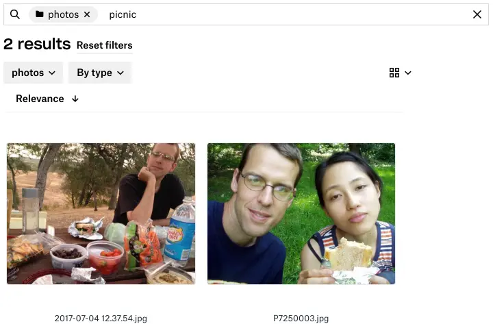
Image content search results for “picnic”
In this post we’ll describe the core idea behind our image content search method, based on techniques from machine learning, then discuss how we built a performant implementation on Dropbox’s existing search infrastructure.
 Dropbox Dash: AI that understands your work
Our approach
Here’s a simple way to state the image search problem: find a relevance function that takes a (text) query q and an image j, and returns a relevance score s indicating how well the image matches the query.
s = f(q, j)
Given this function, when a user does a search we run it on all their images and return those that produce a score above a threshold, sorted by their scores. We build this function using two key developments in machine learning: accurate image classification and word vectors.
Image classification
An image classifier reads an image and outputs a scored list of categories that describe its contents. Higher scores indicate a higher probability that the image belongs to that category.
Categories can be:
- specific objects in the image, such as tree or person
- overall scene descriptors like outdoors or wedding
- characteristics of the image itself, such as black-and-white or close-up
The past decade has seen tremendous progress in image classification using convolutional neural networks, beginning with Krizhevsky et al’s breakthrough result on the ImageNet challenge in 2012. Since then, with model architecture improvements, better training methods, large datasets like Open Images or ImageNet, and easy-to-use libraries like TensorFlow and PyTorch, researchers have built image classifiers that can recognize thousands of categories.
Take a look at how well image classification works today:
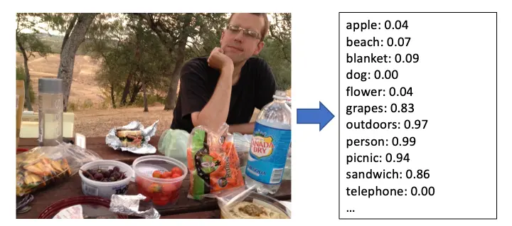
Image classifier outputs for a typical unstaged photo
Image classification lets us automatically understand what’s in an image, but by itself this isn’t enough to enable search. Sure, if a user searches for beach we could return the images with the highest scores for that category, but what if they instead search for shore? What if instead of apple they search for fruit or granny smith?
We could collate a large dictionary of synonyms and near-synonyms and hierarchical relationships between words, but this quickly becomes unwieldy, especially if we support multiple languages.
Word vectors
So let’s reframe the problem. We can interpret the output of the image classifier as a vector jc of the per-category scores. This vector represents the content of the image as a point in C-dimensional category space, where C is the number of categories (several thousand). If we can extract a meaningful representation of the query in this space, we can interpret how close the image vector is to the query vector as a measure of how well the image matches the query.
Fortunately, extracting vector representations of text is the focus of a great deal of research in natural language processing. One of the best known methods in this area is described in Mikolov et al’s 2013 word2vec paper. Word2vec assigns a vector to each word in the dictionary, such that words with similar meanings will have vectors that are close to each other. These vectors are in a d-dimensional word vector space, where d is typically a few hundred.
We can get a vector representation of a search query simply by looking up its word2vec vector. This vector is not in the category space of the image classifier vectors, but we can transform it into category space by referencing the names of the image categories as follows:
- For query word q, get the d-dimensional word vector qw, normalized to a unit vector. We’ll use a w subscript for vectors in word space and a c subscript for vectors in category space.
- For each category, get the normalized word vector for the category name ciw. Then define m̂i = qw · ciw, the cosine similarity between the query vector and the i-th category vector. This score between -1 and 1 indicates how well the query word matches the category name. By clipping negative values to zero, so that mi = max(0, m̂i), we get a score in the same range as the image classifier outputs.
- This lets us calculate qc = [m1 m2 ... mC], a vector in the C-dimensional category space which represents how well the query matches each category, just as the image classifier vector for each image represents how well the image matches each category.
Step 3 is just a vector-matrix multiplication, qc = qwC, where C is the matrix whose columns are the category word vectors ciw.
Once we've mapped the query to category space vector qc, we can take its cosine similarity with the category space vector for each image to get a final relevance score for the image, s = qcjc.
This is our relevance function, and we rank images by this score to show the results of the query. Application of this function to a set of images can also be expressed as a vector-matrix multiplication, s = qcJ, where each column of J is the classifier output vector jc for an image and s is the vector of relevance scores for all images.
An example
Let’s go through an example with only a few dimensions, where word vectors have only three dimensions and the classifier has only four categories: apple, beach, blanket, and dog.
Suppose a user has searched for shore. We look up the word vector to get [0.35 -0.62 0.70], then multiply by the matrix of category word vectors to project the query into category space.
Because the shore word vector is close to the beach word vector, this projection has a large value in the beach category.
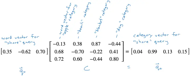
Projecting a query word vector into category space
Modeling details
Our image classifier is an EfficientNet network trained on the OpenImages dataset. It produces scores for about 8500 categories. We’ve found that this architecture and dataset give good accuracy at a reasonable cost, which matters if we want to serve a Dropbox-sized customer base.
We use TensorFlow to train and run the model. We use the pre-trained ConceptNet Numberbatch word vectors. These give good results, and importantly to us they support multiple languages, returning similar vectors for words in different languages with similar meanings. This makes supporting image content search in multiple languages easy: word vectors for dog in English and chien in French are similar, so we can support search in both languages without having to perform an explicit translation.
For multi-word searches, we parse the query as an AND of the individual words. We also maintain a list of multi-word terms like beach ball that can be considered as single words. When a query contains one of these terms we do an alternate parse and run the OR of the two parsed queries—the query beach ball becomes (beach AND ball) OR (beach ball). This will match both large, colorful, inflatable balls and tennis balls in the sand.
Production architecture
It’s not practical to fetch a full, up-to-date J matrix whenever a user does a search. A user may have access to hundreds of thousands or even millions of images, and our classifier outputs are thousands of dimensions, so this matrix could have billions of entries and needs to be updated whenever a user adds, deletes, or modifies an image. This simply won’t scale affordably (yet) for hundreds of millions of users.
So instead of instantiating J for each query, we use an approximation of the method described above, one which can be implemented efficiently on Dropbox’s Nautilus search engine.
Conceptually, Nautilus consists of a forward index that maps each file to some metadata (e.g. the filename) and the full text of the file, and an inverted index that maps each word to a posting list of all the files that contain the word. For text-based search, the index content for a few recipe files might look something like this:
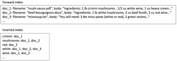
Search index contents for text-based search
If a user searches for white wine, we look up the two words in the inverted index and find that doc_1 and doc_2 have both words, so we should include them in the search results. Doc_3 has only one of the words, so we should either leave it out or put it last in the results list.
Once we've found all the documents we may want to return, we look them up in the forward index and use the information there to rank and filter them. In this case, we might rank doc_1 higher than doc_2 because the two words occur right next to each other.
Repurposing text search methods for image search
We can use this same system to implement our image search algorithm. In the forward index, we can store the category space vector jc of each image. In the inverted index, for each category, we store a posting list of images with positive scores for that category.
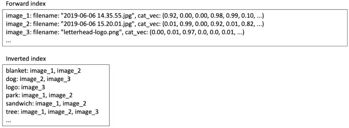
Search index contents for image content search
So, when a user searches for picnic:
- Look up the word vector qw for picnic and multiply by the category space projection matrix C to get qc as described above. C is a fixed matrix that’s the same for all users, so we can hold it in memory.
- For each category with a nonzero entry in qc, fetch the posting list from the inverted index. The union of these lists is the search result set of matching images, but these results still need to be ranked.
- For each search result, fetch the category space vector jc from the forward index and multiply by qc to get the relevance score s. Return results with score above a threshold, ranked by the score.
Optimizing for scalability
This approach is still expensive both in terms of storage space and in query-time processing. If we have 10,000 categories, then for each image we have to store 10,000 classifier scores in the forward index, at a cost of 40 kilobytes if we use four-byte floating point values. And because the classifier scores are rarely zero, a typical image will be added to most of those 10,000 posting lists. If we use four-byte integers for the image ids, that’s another 40 kilobytes, for an indexing cost of 80 kilobytes per image. For many images, the index storage would be larger than the image file!
As for query-time processing — which appears as latency to the user performing the search — we can expect about half of the query-category match scores m̂i to be positive, so we’ll read about 5,000 posting lists from the inverted index. This compares very poorly with text queries, which typically read about ten posting lists.
Fortunately, there are a lot of near-zero values that we can drop to get a much more efficient approximation. The relevance score for each image was given above as s = qcjc, where qc holds the match scores between the query and each of the roughly 10,000 categories, and jc holds the roughly 10,000 category scores from the classifier. Both vectors consist of mostly near-zero values that make very little contribution to s.
In our approximation, we’ll set all but the largest few entries of qc and jc to zero. Experimentally we’ve found that keeping the top 10 entries of qc and top 50 entries of jc is enough to prevent a degradation in quality. The storage and processing savings are substantial:
- In the forward index instead of 10,000-dimensional dense vectors we store sparse vectors with 50 nonzero entries — the top 50 category scores for each image. In a sparse representation we store the position and value of each nonzero entry; 50 two-byte integer positions and 50 four-byte float values requires about 300 bytes.
- In the inverted index, each image is added to 50 posting lists instead of 10,000, at a cost of about 200 bytes. So the total index storage per image is 500 bytes instead of 80 kilobytes.
- At query time, qc has 10 nonzero entries, so we only need to scan 10 posting lists — roughly the same amount of work we do for text queries. This gives us a smaller result set, which we can score more quickly as well.
With these optimizations, indexing and storage costs are reasonable, and query latencies are on par with those for text search. So when a user initiates a search we can run both text and image searches in parallel, and show the full set of results together, without making the user wait any longer than they would for a text-only search.
Current deployment
Image content search is currently enabled for all of our Professional and Business level users. We combine image content search for general images, OCR-based search for images of documents, and full-text search for text documents to make most of these users' files available through content-based search.
Video search?
Of course, we’re working to let you search all of your Dropbox content. Image search is a big step toward that. Eventually, we hope to be able to search video content as well. The techniques to find one frame in a video, or to index an entire clip for searching, perhaps by adapting still image techniques, are still at the research stage, but it was just a few years ago that “find all the photos from my picnic with my dog in them” only worked in Hollywood movies.
Our goal is: If it’s in your Dropbox, we’ll find it for you!


