Magic Pocket is the core Dropbox storage system—a custom-built, exabyte-scale blob storage system designed for durability, availability, scale, and efficiency. It holds user content, which means it must be safe, fast, and cost-effective to scale with the company. For Dropbox, storage efficiency really matters. We measure it by looking at how much total disk space we use compared to how much user data we’re actually storing.
Last year, we rolled out a new service that changed how data is placed across Magic Pocket. The change reduced write amplification for background writes, so each write triggered fewer backend storage operations. But it also had an unintended side effect: fragmentation increased, pushing storage overhead higher. Most of that growth came from a small number of severely under-filled volumes that consumed a disproportionate share of raw capacity, and our existing compaction strategy couldn’t reclaim the space quickly enough. At exabyte scale, even modest increases in overhead translate into meaningful infrastructure and capacity costs, so bringing that number back down quickly became a priority.
In this post, we’ll walk through why overhead is particularly hard to control in an immutable blob store, how compaction works in Magic Pocket, and the multi-strategy approach we rolled out to drive overhead back down, even below our previous baseline.
 Dropbox Dash: AI that understands your work
The cost of immutability
When users upload files to Dropbox, Magic Pocket breaks those files into smaller pieces called blobs and stores them across its storage fleet. A blob is simply a chunk of binary data—part or all of a user file—written to disk. Magic Pocket is an immutable blob store, which means that once a blob is written, it is never modified in place. If a file is updated or deleted, new data is written and the old data remains until it is reclaimed by a compaction process.
At Dropbox scale, Magic Pocket stores trillions of blobs and processes millions of deletes each day. (A delete is a request to remove a blob when a file is deleted or updated.) Because data is immutable, deletes do not immediately free up disk space. Old data stays on-disk inside storage volumes. Once a volume is closed, it is never reopened. The tradeoff is that deletes leave unused space behind, and that waste grows over time unless we actively reclaim it.
Without reclamation, volumes gradually become partially filled, spreading live data across more disks than necessary. Fragmentation from lack of reclamation can have a big impact on storage overhead.
We address this in two steps. Garbage collection identifies blobs that are no longer referenced and marks them as safe to remove, but it does not free space on its own. Compaction performs the physical reclamation. Because volumes cannot be modified once closed, we gather the live blobs from volumes, write them into new volumes, and retire the old ones. This is how deletes eventually translate into reusable space.
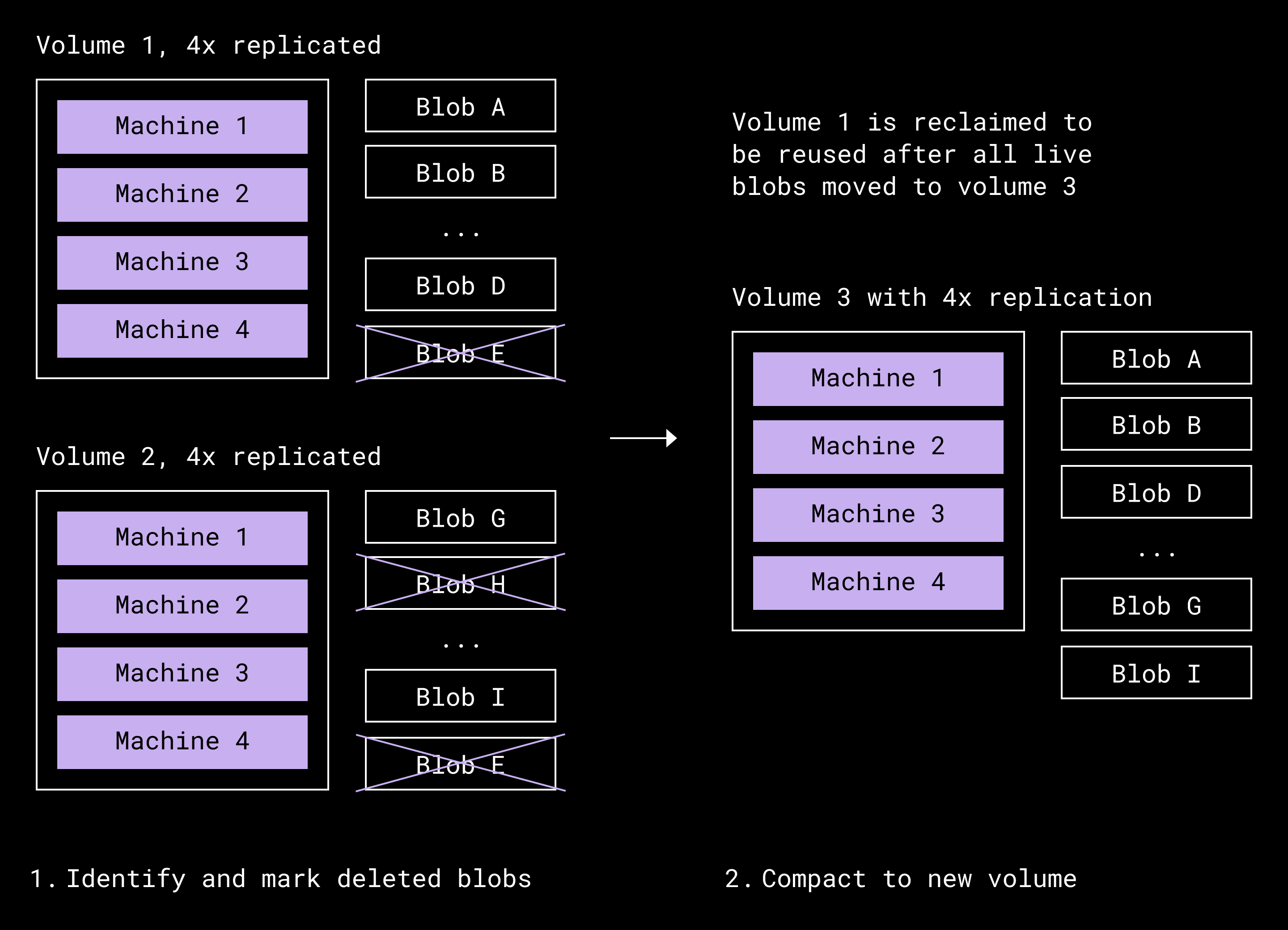
Compaction lifecycle of volume 1 getting compacted along with a donor volume (2). Volume 1 is then eligible to be reused.
Compaction controls the waste created by deletes. But fragmentation isn’t the only factor that affects storage overhead—durability does too. To protect against hardware failures, we store data redundantly either as full copies or as encoded fragments distributed across different machines, so data can be recovered after disk or server failures. One approach is replication, which keeps multiple full copies of each blob and increases storage use proportionally. In Magic Pocket, we use erasure coding for nearly all data. Erasure coding splits data into fragments and adds a small number of parity fragments (extra pieces that let us reconstruct the original data if part of it is lost). It provides the same level of fault tolerance as replication, but with significantly less additional storage.
Redundancy affects overhead, but fragmentation determines how efficiently that space is used. A useful way to think about this is what percentage of a volume that contains active data. If a volume is half full of live data, we are effectively using twice the storage needed for that data. If only ten percent is live, we are using about ten times the space required. Without continuous compaction, disk capacity would eventually be exhausted even if the data redundancy scheme—how we store extra copies or fragments to protect against failures—never changed. Keeping storage overhead low in an immutable system therefore requires both efficient redundancy and constant consolidation of fragmented space.
The incident that forced a rethink
Earlier this year, we uncovered an issue with a new service that performs on-the-fly erasure coding, which we’ll refer to as the Live Coder service. It rolled out gradually over several months to new regions. The problem, which went unnoticed for weeks, was that volumes created through this path were severely under-filled. In the worst cases, less than five percent of their allocated capacity contained live data.
In practical terms, that meant live data was spread across far more volumes than intended. Instead of densely packing blobs together, we were creating many mostly empty volumes. Because volumes are fixed in size, each under-filled volume consumed the same disk allocation as a full one. The result was a sharp increase in fragmentation and a corresponding rise in storage overhead.
We saw early signs that this was impacting our effective replication factor, a signal that more raw storage was being consumed per live byte than expected. But identifying the root cause required significant investigation. Once we understood what was happening, we also needed to design recovery mechanisms capable of bringing overhead back down efficiently. The existing compaction strategy continued to make progress, but it was not designed to handle a long tail of severely under-filled volumes at this scale.
This incident exposed a limitation in our steady-state approach. It forced us to rethink how compaction should work when the distribution of live data shifts, and to develop new strategies capable of reclaiming space faster and more effectively.
What steady-state compaction looks like
In normal operation, before the incident, the distribution of data across volumes was relatively stable. Most volumes were already highly filled, and deletes accumulated gradually. In that steady state, compaction’s job was to continuously consolidate small amounts of fragmentation and keep storage overhead bounded.
For years, our baseline compaction strategy, which we call L1, worked well in this environment. It treats compaction as a packing problem: move live data from one or more partially filled donor volumes into a host volume that has enough free space. Over time, as donor volumes are drained of their live data, they become empty and can be removed.
L1 selects a host volume that is already highly filled, then chooses donor volumes whose live bytes fit into the host’s available space, and finally, writes them into a new volume. The selection logic is simple and fast, and it keeps placement risk and metadata updates bounded. However, each compaction run is relatively expensive. It may read tens of GiB across the host and donors but typically produces only a single new densely packed volume. On average, fewer than one full volume is reclaimed per run, since only donors are fully drained.
This approach works well when most volumes are close to full. But the incident changed that distribution. We saw overhead concentrated in a long tail of severely under-filled volumes. L1 continued to make progress, but it could not compact those volumes quickly enough. Its core assumption, that most volumes are highly filled, no longer held. To address this, we introduced two new compaction strategies, L2 and L3, each designed to handle different parts of the volume fill distribution.
A better way to reclaim space
When the distribution shifted, the limitations of L1 became clear. It was designed to top off already dense volumes, not to quickly reclaim a large population of severely under-filled ones. We needed a strategy that could reclaim space faster by combining multiple sparse volumes into a single near-full destination.
When we examined the distribution of live data across volumes, most of the wasted space was concentrated in a distinct subset that was less than half full. L1 wasn’t designed for this pattern; it topped off already dense volumes rather than aggressively consolidating sparse ones. Instead of incrementally packing donors into a host, L2 groups under-filled volumes together and selects combinations whose live data can nearly fill a new destination volume. Reclaiming several sparse volumes at once allows the system to recover space far more quickly.
Inputs:
volumes[] with LiveBytes
  maxVolBytes (destination volume capacity)
  maxVolumesToUse (count cap)
  granularity (scaling factor)
1) Scale live bytes and capacity by granularity to shrink the DP table.
2) DP over (i = volume index, k = count, c = capacity), keeping max packed bytes.
3) Track choices in a parallel “choice” table for reconstruction.
4) Backtrack from the best (k, capacity) to recover the selected volumes.
Under the hood, L2 is a bounded packing problem solved with dynamic programming. For each run, we choose a limited set of volumes whose combined live bytes come as close as possible to the destination capacity without exceeding it. To keep this practical at production scale, we cap how many source volumes can be used in one run and coarsen byte counts to reduce the search space. This keeps compute and memory bounded while still producing tight packings.
In practice, we tuned granularity, batch size, and planner concurrency to balance packing quality against compute and memory cost. Those settings allowed L2 to run efficiently in production while still producing tight packings.
In testing, the results were strong. With data shaped to resemble production distributions, L2 consistently produced near-full volumes. In production, it reduced compaction overhead two to three times faster than L1. In cells where L2 was enabled, overhead returned to sustainable levels within days, and over the course of a week, compaction overhead was thirty to fifty percent lower compared to cells running L1 alone. (Cells, in this instance, refer to independent units of the storage system that manage their own data.)
Cleaning up the sparsest volumes
L2 was effective at targeting the middle of the distribution, where volumes were under-filled but still dense enough to combine efficiently. But it was less effective at quickly reclaiming the sparsest volumes, or those with only a small fraction of live data remaining. These volumes formed the extreme tail of the distribution and required a different approach.
While iterating on compaction strategies, we returned to the Live Coder service. Its original purpose was to write data directly into erasure-coded volumes, bypassing the initial replicated write path. Although it isn’t ideal for latency-sensitive traffic, it’s well suited for background workflows where throughput matters more than immediacy.
Compaction is, in effect, a constrained form of re-encoding: take live data from one set of volumes and produce a new, durable volume. L3 builds on that idea by using Live Coder as a streaming pipeline. Instead of packing volumes together in a bounded batch, L3 continuously feeds the remaining live blobs from severely under-filled volumes into Live Coder and allows it to accumulate and encode them into new volumes over time. Once a source volume’s live data has been drained, it can be reclaimed immediately.
This strategy focuses on volumes that aren’t good candidates for L1 or L2. Under-filled volumes occur naturally as donors are partially drained, and they can accumulate quickly during failure modes like the incident described earlier. By prioritizing the sparsest volumes first, L3 minimizes the amount of data that needs to be rewritten per reclaimed volume and accelerates recovery of fragmented space.
L3 does introduce tradeoffs. Because it writes live data into entirely new volumes, every blob it moves has to be rewritten, which means new identifiers and additional metadata updates. That extra bookkeeping creates load on storage and metadata systems. With the amount of under-filled volumes observed in steady state, that additional load is tolerable and limits are in place to prevent overwhelming those systems.
Operational tuning and safeguards
To prevent compaction from competing with user traffic, we rate-limit the pipeline and keep traffic local to each cell rather than sending it across data centers. Together, L1, L2, and L3 form a layered strategy: L1 maintains steady state, L2 consolidates moderately under-filled volumes, and L3 drains the sparsest tail, thereby reclaiming space quickly without destabilizing the fleet.
Rolling out L2 and L3 wasn’t just about improving packing efficiency. We also had to ensure the system could absorb the additional work without creating new bottlenecks. Compaction touches storage, compute, metadata systems, and network bandwidth, so increasing its aggressiveness requires careful controls.
One of the most sensitive levers is the host eligibility threshold, which determines when a volume qualifies for compaction. If the threshold is too high, too few volumes are eligible and overhead rises. If it’s too low, we spend compute and I/O reclaiming very little space. We replaced static tuning with a dynamic control loop that adjusts the threshold based on fleet signals. When overhead rises, the system raises the threshold to prioritize higher-yield compactions. When overhead stabilizes, it lowers the threshold to stay responsive to deletes without over-compacting.
Candidate ordering is another important tuning lever. Choosing which volumes to compact first can speed up space reclamation, but it can also increase metadata work because more blobs may need to be rewritten. We tailor the ordering to each strategy. L1 stays conservative and limits how many donor volumes it touches to keep placement risk and metadata load low. L2 benefits from more aggressive grouping because denser packings reclaim more space per compaction run. L3 focuses on the sparsest volumes first, since draining them typically requires rewriting relatively little data per volume.
The final step was enabling L1, L2, and L3 to run concurrently without interfering with one another. Each strategy targets a different part of the volume distribution: L1 maintains steady state among highly filled volumes, L2 targets moderately under-filled volumes into dense destinations, and L3 drains the sparsest volumes. We enforce clear eligibility boundaries between strategies and rate-limit each path to protect downstream services. We also constrain traffic locality so compaction remains within a cell and avoids stressing cross-cluster bandwidth.
Together, these safeguards allow the system to adapt to workload shifts while keeping metadata pressure, network traffic, and compute utilization within safe limits.
What we learned
This project reinforced that compaction can’t rely on a single heuristic. L1 worked well in steady state because most volumes were already close to full, and only a small number were partially filled at any given time. When that distribution shifted and a large group of very sparsely filled volumes accumulated, L1 couldn’t recover overhead quickly enough. Splitting the problem across multiple strategies gave us coverage across the full range of volume fill levels: L1 maintains steady state for mostly full volumes, L2 consolidates moderately under-filled volumes, and L3 focuses on the sparsest volumes.
We also learned that manual tuning doesn’t scale. The host eligibility threshold is too sensitive to manage by hand, especially at exabyte scale. Moving to a dynamic control loop tied to fleet signals made overhead more stable and reduced the need for constant intervention. Candidate ordering and rate limits must also be tuned with awareness of downstream systems, particularly metadata services.
Operationally, metadata capacity turned out to be one of our biggest constraints. Not every compaction move has the same metadata cost. In L1 and L2, many blobs can stay under the same volume identity, so only donor blobs need location rewrites. In L3, blobs are written into brand-new volumes, so most blobs need new location entries. So it wasn’t enough to pack volumes efficiently; we also had to control how much rewriting we triggered. By limiting how much work L2 does in a single run, routing the sparsest volumes through L3, and keeping traffic local to each cell, we were able to reclaim space without overwhelming our metadata, storage, or network systems.
Finally, this work showed us that we needed better visibility into how compaction was performing. We added metrics to track how much data Live Coder is producing, how full volumes are across the fleet, and how storage overhead changes week over week. We also put monitoring in place to warn us early if compaction starts to fall behind. The goal is to catch shifts in how data is distributed before overhead rises too far so that we can respond proactively instead of scrambling to recover later.
Storage overhead directly determines how much raw capacity we need in order to store the same amount of live user data. Even small changes in overhead materially affect hardware purchases and fleet growth. By turning compaction into a layered, adaptive pipeline and strengthening our monitoring and controls, we made Magic Pocket more resilient to workload changes and better positioned to keep storage growth predictable over time.
Acknowledgments: Tommy Dean (contributions to L2 strategy) and Lisa Kosiachenko (contributions on automation)
~ ~ ~
If building innovative products, experiences, and infrastructure excites you, come build the future with us! Visit jobs.dropbox.com to see our open roles.


